MAGNETIC  QUANTUM  NUMBERS

We have now described the orbital angular momentum of an electron with the term l, but an electron with angular momentum is analogous to a current loop and will exhibit a magnetic moment. This magnetic moment will (generally speaking) be characterized by the magnetic quantum number m_l. An alternative way to think about this parameter is that it represents the direction of angular momentum of an electron. Assuming that we’ve chosen an axis for the atom, the orientation of this angular momentum (or orbital) with respect to this axis gives rise to ml. It can be thought of as the three-dimensional tilt of an elliptical orbit, as depicted in Figure1.1. This number is confined by the orbital quantum number l and may assume integer values ranging from -l to ‏l. For example, an s orbital with l = 0 always assumes a magnetic quantum number of m_l =0, while a p orbital with l =1 can have numbers m_l = -1, 0, or ‏1. The range of numbers increases as the orbital does, with five values possible for a d orbital, and so on. In all, there are -l‏+1 possible values for ml for a given value of l.

    It is somewhat puzzling perhaps why this is called the magnetic quantum number as opposed to tilt or some other description. The answer lies in the conditions

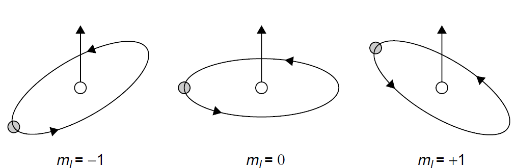
Figure 1.1. Representation of the magnetic quantum number.

Figure 1.2. Zeeman effect on the red hydrogen line (energy levels and resulting spectra).

required to produce an energy difference between levels with various values for ml. Under the influence of a magnetic field, certain spectral emission lines can be split into a number of hyperfine lines in what is called the Zeeman effect. Figure 1.2 depicts the effect of an external magnetic field on the red emission line of hydrogen.                

       With no external magnetic field, the transition looks like a simple one between the n =3 and n =2 levels, resulting in the emission of a single wavelength. When a magnetic field is applied, the alignment of various magnetic moments becomes apparent as a number of spectra lines appear. Although it appears from Figure 1.2 that many hyperfine transitions are possible, there are selection rules that determine which transitions are unlikely (called forbidden) and which are allowed. The simple rule is that a transition is allowed (i.e., is quite probable) if the change in orbital angular momentum (l) is 21 or ‏1 (but not zero). A transition is also allowed if the change in the magnetic quantum number (m_l) is -1, 0, or ‏1. Referring back to the figure, it is apparent that the transition from n =3, m_l = ‏+2 to n = 2, m_l =+ ‏1 obeys these rules but that no other transition originating from the n = 3, m_l =+2 level will. Furthermore, only three spectral lines are visible in the split because there are only three unique hyperfine transitions (i.e., changes in quantum numbers). Further application of selection rules can be seen in the spectrum of sodium observed, in which observed transitions correspond to a jump between an s and a p orbital (a change in l of 1) but never from a p to another p orbital.

مواضيع ذات صلة

الفزياء والكون .. ميكانيكا الكم

ميكانيكا الكم الخاصة بالروابط

ما الفائدة؟

إعادة النظر في اللامحلية

عوالم متعدّدة

هل نغيّر الفيزياء؟

الاحتمالات والقياسات

مبرهنة بيل وضرورة اللامحلية

الترابط والتشابك

الحالات الكمية والتراكب الكمي

التداخل والقياس

ألغاز الكم