The semiclassical laser equations for the macroscopic quantities electric field strength, polarization and inversion density in the rotating wave- and slowly varying amplitude approximation

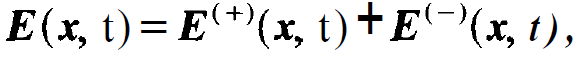
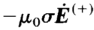
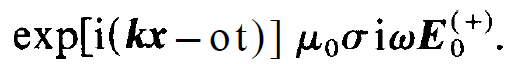
The rotating wave approximation and the slowly varying amplitude approximation cannot only be applied to the laser equations in a resonator, but they may also serve to simplify the laser equations. Since we shall need the thus resulting equations much later in this book, the reader may skip this section and read it only later when it will be needed. We start with the field. With respect to its 1.h.s. we have several options depending on the specific problem, i.e. standing or running waves. When we use standing waves, we are essentially dealing with the field in a resonator. Since this problem, we shall deal here with running waves. Incidentally, this allows us to treat the functional dependence of E on x and t in a symmetric fashion. To this end we consider a plane wave exp[i(kx- i⍵t)] which is slowly modulated in time and space. We therefore write

 (1 .1)

where

    (1.2)

and

    (1.3)

We form

     (1.4)

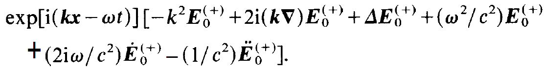
and insert (1.2) in (1.4). This yields

 (1.5)

In the square brackets, the first and fourth term cancel each other, while the third and sixth term can be neglected due to the slowly varying amplitude approximation. In this way (1.4) reduces to

 (1.6)

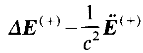
In a similar, though simpler fashion, we reduce

     (1.7)

to

 (1.8)

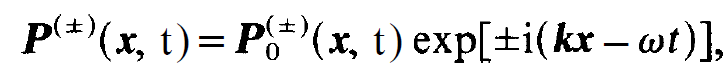
In order to transform the r.h.s. we assume P^(±) (x, t) in the same form as E^(±)(x , t), i.e.

 (1.9)

where P₀^(±)  is a function which varies much more slowly in space and time than exp[±i(kx - ⍵t)]. Applying the slowly varying amplitude approximation to μ₀ P^(±) (x, t), we readily obtain

   (1.10)

We now split the r.h.s. and the 1.h.s. their positive and negative frequency parts, respectively, and collect the corresponding terms (1.6), (1.8) and (1.10). After dividing the resulting equation by exp[i(kx - ⍵t)] we obtain

 (1.11)

In the last step of our analysis, we multiply this equation by c²/(2iw), use the relations

    (1.12)

and on the r.h.s. of (1.11) the approximation ⍵≈ . This leaves us with the final result, namely the field equation for the slowly varying amplitude

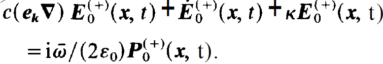    (1.13)

We immediately obtain the equation for the slowly varying amplitude of the polarization

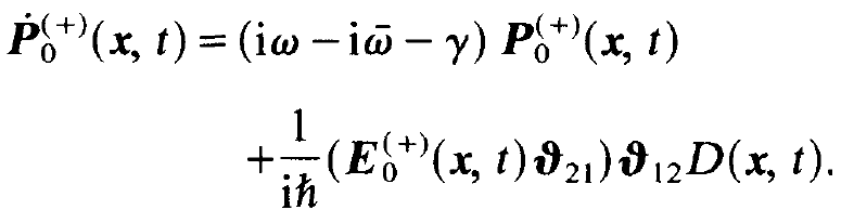    (1.14)

Note that  need not coincide with ⍵, but that we require only | - ⍵|< <⍵, . We insert (1.1), (1.2) and (1.10). When we neglect in

    (1.15)

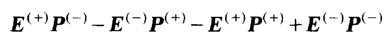
the rapidly oscillating terms  exp[±i(⍵ +)t] we can into the equation for the inversion density containing only slowly varying amplitudes

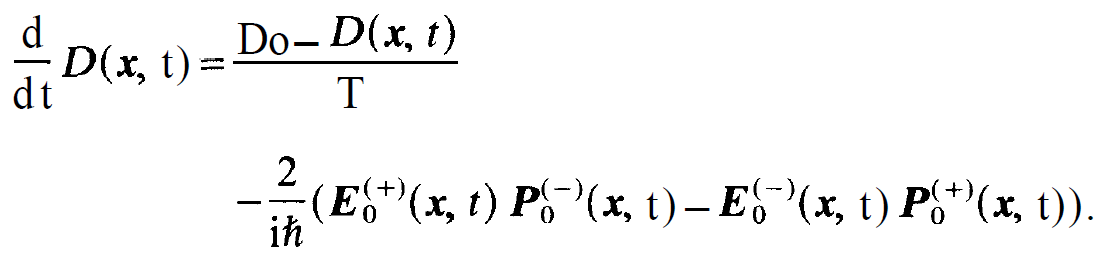 (1.16)

The equations (1.3), (1.4) and (1.16) represent our final result.

مواضيع ذات صلة

الليزرات والسوائل التي تصعد إلى الأعلى

الليزر والميزر

Flashtube Explosion

Tube Failure

Plane–Parallel Resonator

Concave–Convex Resonator

Plano-Concave Resonator

Mirrors of Equal Curvature

Parasitic Oscillations

Prelasing

Depopulation Losses

The Three-Level System