0
EN
1
المرجع الالكتروني للمعلوماتية

تاريخ الرياضيات

الاعداد و نظريتها

تاريخ التحليل

تار يخ الجبر

الهندسة و التبلوجي

الرياضيات في الحضارات المختلفة

العربية

اليونانية

البابلية

الصينية

المايا

المصرية

الهندية

الرياضيات المتقطعة

المنطق

اسس الرياضيات

فلسفة الرياضيات

مواضيع عامة في المنطق

الجبر

الجبر الخطي

الجبر المجرد

الجبر البولياني

مواضيع عامة في الجبر

الضبابية

نظرية المجموعات

نظرية الزمر

نظرية الحلقات والحقول

نظرية الاعداد

نظرية الفئات

حساب المتجهات

المتتاليات-المتسلسلات

المصفوفات و نظريتها

المثلثات

الهندسة

الهندسة المستوية

الهندسة غير المستوية

مواضيع عامة في الهندسة

التفاضل و التكامل

المعادلات التفاضلية و التكاملية

معادلات تفاضلية

معادلات تكاملية

مواضيع عامة في المعادلات

التحليل

التحليل العددي

التحليل العقدي

التحليل الدالي

مواضيع عامة في التحليل

التحليل الحقيقي

التبلوجيا

نظرية الالعاب

الاحتمالات و الاحصاء

نظرية التحكم

بحوث العمليات

نظرية الكم

الشفرات

الرياضيات التطبيقية

نظريات ومبرهنات

علماء الرياضيات

500AD

500-1499

1000to1499

1500to1599

1600to1649

1650to1699

1700to1749

1750to1779

1780to1799

1800to1819

1820to1829

1830to1839

1840to1849

1850to1859

1860to1864

1865to1869

1870to1874

1875to1879

1880to1884

1885to1889

1890to1894

1895to1899

1900to1904

1905to1909

1910to1914

1915to1919

1920to1924

1925to1929

1930to1939

1940to the present

علماء الرياضيات

الرياضيات في العلوم الاخرى

بحوث و اطاريح جامعية

هل تعلم

طرائق التدريس

الرياضيات العامة

نظرية البيان

قم بتسجيل الدخول اولاً لكي يتسنى لك الاعجاب والتعليق.

Uniform Distribution

المؤلف:  Beyer, W. H.

المصدر:  CRC Standard Mathematical Tables, 28th ed. Boca Raton, FL: CRC Press

الجزء والصفحة:  pp. 531 and 533

15-4-2021

2554

+

-

20

Uniform Distribution

A uniform distribution, sometimes also known as a rectangular distribution, is a distribution that has constant probability.
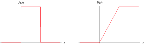
UniformDistribution

The probability density function and cumulative distribution function for a continuous uniform distribution on the interval [a,b] are

P(x) = <span style={0 for x<a; 1/(b-a) for a<=x<=b; 0 for x>b" src="https://mathworld.wolfram.com/images/equations/UniformDistribution/Inline4.gif" style="height:82px; width:124px" />

(1)

D(x) = <span style={0 for x<a; (x-a)/(b-a) for a<=x<=b; 1 for x>b." src="https://mathworld.wolfram.com/images/equations/UniformDistribution/Inline7.gif" style="height:78px; width:124px" />

(2)

These can be written in terms of the Heaviside step function H(x) as

P(x) = (H(x-a)-H(x-b))/(b-a)

(3)

D(x) = ((x-a)H(x-a)-(x-b)H(x-b))/(b-a),

(4)

the latter of which simplifies to the expected D(x)=(x-a)/(b-a) for a<x<b.

The continuous distribution is implemented as UniformDistribution[ab].

For a continuous uniform distribution, the characteristic function is

 phi(t)=2/((b-a)t)sin[1/2(b-a)t]e^(i(a+b)t/2).

(5)

If a=0 and b=1, the characteristic function simplifies to

phi(t) = (2sin(1/2t)e^(it/2))/t

(6)

= (i-icost+sint)/t.

(7)

The moment-generating function is

M(t) = <e^(xt)>

(8)

= int_a^b(e^(xt))/(b-a)dx=[(e^(xt))/(t(b-a))]_a^b

(9)

= <span style={(e^(tb)-e^(ta))/(t(b-a)) for t!=0; 1 for t=0," src="https://mathworld.wolfram.com/images/equations/UniformDistribution/Inline33.gif" style="height:66px; width:125px" />

(10)

and

= 1/(b-a)[1/t(be^(bt)-ae^(at))-1/(t^2)(e^(bt)-e^(at))]

(11)

= (e^(bt)(bt-1)-e^(at)(at-1))/((b-a)t^2).

(12)

The moment-generating function is not differentiable at zero, but the moments can be calculated by differentiating and then taking lim_(t->0). The raw moments are given analytically by

= int_(-infty)^infty(H(x-a)-H(x-b))/(b-a)x^ndx

(13)

= int_a^b(x^n)/(b-a)dx

(14)

= (b^(n+1)-a^(n+1))/((n+1)(b-a)).

(15)

The first few are therefore given explicitly by

= 1/2(a+b)

(16)

= 1/3(a^2+ab+b^2)

(17)

= 1/4(a+b)(a^2+b^2)

(18)

= 1/5(a^4+a^3b+a^2b^2+ab^3+b^4).

(19)

The central moments are given analytically by

= int_(-infty)^infty(H(x-a)-H(x-b))/(b-a)[x-1/2(a+b)]^ndx

(20)

= int_a^b([x-1/2(a+b)]^n)/(b-a)dx

(21)

= ((a-b)^n+(b-a)^n)/(2^(n+1)(n+1)).

(22)

The first few are therefore given explicitly by

mu_1 = 0

(23)

mu_2 = 1/(12)(b-a)^2

(24)

mu_3 = 0

(25)

mu_4 = 1/(80)(b-a)^4.

(26)

The mean, variance, skewness, and kurtosis excess are therefore

mu = 1/2(a+b)

(27)

sigma^2 = 1/(12)(b-a)^2

(28)

gamma_1 = 0

(29)

gamma_2 = -6/5.

(30)


REFERENCES:

Beyer, W. H. CRC Standard Mathematical Tables, 28th ed. Boca Raton, FL: CRC Press, pp. 531 and 533, 1987.

اشترك بقناتنا على التلجرام ليصلك كل ما هو جديد