

 تاريخ الرياضيات
 الرياضيات في الحضارات المختلفة
 الرياضيات المتقطعة
 الجبر
الجبر
 الهندسة
 المعادلات التفاضلية و التكاملية
 التحليل
 علماء الرياضيات
 |
Read More
Date: 7-3-2021
Date: 15-4-2021
Date: 6-2-2016
|

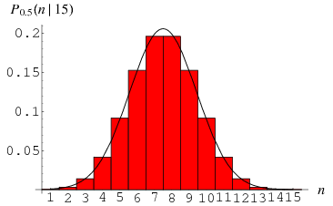
A normal distribution in a variate  with mean
  and variance
  is a statistic distribution with probability density function
 |
(1) |
on the domain  . While statisticians and mathematicians uniformly use the term "normal distribution" for this distribution, physicists sometimes call it a Gaussian distribution and, because of its curved flaring shape, social scientists refer to it as the "bell curve." Feller (1968) uses the symbol
  for
for  in the above equation, but then switches to
  in Feller (1971).
de Moivre developed the normal distribution as an approximation to the binomial distribution, and it was subsequently used by Laplace in 1783 to study measurement errors and by Gauss in 1809 in the analysis of astronomical data (Havil 2003, p. 157).
The normal distribution is implemented in the Wolfram Language as NormalDistribution[mu, sigma].
The so-called "standard normal distribution" is given by taking  and
and  in a general normal distribution. An arbitrary normal distribution can be converted to a standard normal distribution by changing variables to
  , so
, so  , yielding
 |
(2) |
The Fisher-Behrens problem is the determination of a test for the equality of means for two normal distributions with different variances.
The normal distribution function  gives the probability that a standard normal variate assumes a value in the interval
 ![[0,z]](https://mathworld.wolfram.com/images/equations/NormalDistribution/Inline13.gif) ,
,
 |
 |
 |
(3) |
 |
 |
 |
(4) |
where erf is a function sometimes called the error function. Neither  nor erf can be expressed in terms of finite additions, subtractions, multiplications, and root extractions, and so both must be either computed numerically or otherwise approximated.

The normal distribution is the limiting case of a discrete binomial distribution  as the sample size
  becomes large, in which case
  is normal with mean and variance
 |
 |
 |
(5) |
 |
 |
 |
(6) |
with  .
.
The distribution  is properly normalized since
 |
(7) |
The cumulative distribution function, which gives the probability that a variate will assume a value  , is then the integral of the normal distribution,
 |
 |
 |
(8) |
 |
 |
 |
(9) |
 |
 |
![1/2[1+erf((x-mu)/(sigmasqrt(2)))],](https://mathworld.wolfram.com/images/equations/NormalDistribution/Inline41.gif) |
(10) |
where erf is the so-called error function.
Normal distributions have many convenient properties, so random variates with unknown distributions are often assumed to be normal, especially in physics and astronomy. Although this can be a dangerous assumption, it is often a good approximation due to a surprising result known as the central limit theorem. This theorem states that the mean of any set of variates with any distribution having a finite mean and variance tends to the normal distribution. Many common attributes such as test scores, height, etc., follow roughly normal distributions, with few members at the high and low ends and many in the middle.
Because they occur so frequently, there is an unfortunate tendency to invoke normal distributions in situations where they may not be applicable. As Lippmann stated, "Everybody believes in the exponential law of errors: the experimenters, because they think it can be proved by mathematics; and the mathematicians, because they believe it has been established by observation" (Whittaker and Robinson 1967, p. 179).
Among the amazing properties of the normal distribution are that the normal sum distribution and normal difference distribution obtained by respectively adding and subtracting variates  and
and  from two independent normal distributions with arbitrary means and variances are also normal! The normal ratio distribution obtained from
  has a Cauchy distribution.
Using the k-statistic formalism, the unbiased estimator for the variance of a normal distribution is given by
 |
(11) |
where
 |
(12) |
so
 |
(13) |
The characteristic function for the normal distribution is
 |
(14) |
and the moment-generating function is
 |
 |
 |
(15) |
 |
 |
 |
(16) |
 |
 |
 |
(17) |
so
 |
 |
 |
(18) |
 |
 |
 |
(19) |
and
 |
 |
 |
(20) |
 |
 |
 |
(21) |
These can also be computed using
 |
 |
![ln[M(t)]=mut+1/2sigma^2t^2](https://mathworld.wolfram.com/images/equations/NormalDistribution/Inline68.gif) |
(22) |
 |
 |
 |
(23) |
 |
 |
 |
(24) |
yielding, as before,
 |
 |
 |
(25) |
 |
 |
 |
(26) |
The raw moments can also be computed directly by computing the raw moments  ,
,
 |
(27) |
(Papoulis 1984, pp. 147-148). Now let
 |
 |
 |
(28) |
 |
 |
 |
(29) |
 |
 |
 |
(30) |
giving the raw moments in terms of Gaussian integrals,
 |
(31) |
Evaluating these integrals gives
 |
 |
 |
(32) |
 |
 |
 |
(33) |
 |
 |
 |
(34) |
 |
 |
 |
(35) |
 |
 |
 |
(36) |
Now find the central moments,
 |
 |
 |
(37) |
 |
 |
 |
(38) |
 |
 |
 |
(39) |
 |
 |
 |
(40) |
The variance, skewness, and kurtosis excess are given by
 |
 |
 |
(41) |
 |
 |
 |
(42) |
 |
 |
 |
(43) |
The cumulant-generating function for a normal distribution is
 |
 |
 |
(44) |
 |
 |
 |
(45) |
so
 |
 |
 |
(46) |
 |
 |
 |
(47) |
 |
 |
 |
(48) |
For normal variates,  for
for  , so the variance of k-statistic
  is
is
 |
 |
 |
(49) |
 |
 |
 |
(50) |
Also,
 |
 |
 |
(51) |
 |
 |
 |
(52) |
 |
 |
 |
(53) |
where
 |
 |
 |
(54) |
 |
 |
 |
(55) |
The variance of the sample variance  for a general distribution is given by
![var(s^2)=((N-1)[(N-1)mu_4-(N-3)mu_2^2])/(N^3),](https://mathworld.wolfram.com/images/equations/NormalDistribution/NumberedEquation10.gif) |
(56) |
which simplifies in the case of a normal distribution to
 |
(57) |
(Kenney and Keeping 1951, p. 164).
If  is a normal distribution, then
![D(x)=1/2[1+erf((x-mu)/(sigmasqrt(2)))],](https://mathworld.wolfram.com/images/equations/NormalDistribution/NumberedEquation12.gif) |
(58) |
so variates  with a normal distribution can be generated from variates
  having a uniform distribution in (0,1) via
 |
(59) |
However, a simpler way to obtain numbers with a normal distribution is to use the Box-Muller transformation.
The differential equation having a normal distribution as its solution is
 |
(60) |
since
 |
(61) |
 |
(62) |
 |
(63) |
This equation has been generalized to yield more complicated distributions which are named using the so-called Pearson system.
The normal distribution is also a special case of the chi-squared distribution, since making the substitution
 |
(64) |
gives
 |
 |
 |
(65) |
 |
 |
 |
(66) |
Now, the real line  is mapped onto the half-infinite interval
  by this transformation, so an extra factor of 2 must be added to
  , transforming
  into
into
 |
 |
 |
(67) |
 |
 |
 |
(68) |
(Kenney and Keeping 1951, p. 98), where use has been made of the identity  . As promised, (68) is a chi-squared distribution in
  with
with  (and also a gamma distribution with
  and
and  ).
).
REFERENCES:
Beyer, W. H. CRC Standard Mathematical Tables, 28th ed. Boca Raton, FL: CRC Press, pp. 533-534, 1987.
Feller, W. An Introduction to Probability Theory and Its Applications, Vol. 1, 3rd ed. New York: Wiley, 1968.
Feller, W. An Introduction to Probability Theory and Its Applications, Vol. 2, 3rd ed. New York: Wiley, p. 45, 1971.
Havil, J. Gamma: Exploring Euler's Constant. Princeton, NJ: Princeton University Press, p. 157, 2003.
Kenney, J. F. and Keeping, E. S. Mathematics of Statistics, Pt. 2, 2nd ed. Princeton, NJ: Van Nostrand, 1951.
Kraitchik, M. "The Error Curve." §6.4 in Mathematical Recreations. New York: W. W. Norton, pp. 121-123, 1942.
Papoulis, A. Probability, Random Variables, and Stochastic Processes, 2nd ed. New York: McGraw-Hill, pp. 100-101, 1984.
Patel, J. K. and Read, C. B. Handbook of the Normal Distribution. New York: Dekker, 1982.
Spiegel, M. R. Theory and Problems of Probability and Statistics. New York: McGraw-Hill, pp. 109-111, 1992.
Steinhaus, H. Mathematical Snapshots, 3rd ed. New York: Dover, pp. 285-290, 1999.
Whittaker, E. T. and Robinson, G. "Normal Frequency Distribution." Ch. 8 in The Calculus of Observations: A Treatise on Numerical Mathematics, 4th ed. New York: Dover, pp. 164-208, 1967.


|
|
|
|
دراسة: حفنة من الجوز يوميا تحميك من سرطان القولون
|
|
|
|
|
|
|
تنشيط أول مفاعل ملح منصهر يستعمل الثوريوم في العالم.. سباق "الأرنب والسلحفاة"
|
|
|
|
|
|
|
الطلبة المشاركون: مسابقة فنِّ الخطابة تمثل فرصة للتنافس الإبداعي وتنمية المهارات
|
|
|