
The vector model
 المؤلف:
Peter Atkins، Julio de Paula
المؤلف:
Peter Atkins، Julio de Paula
 المصدر:
ATKINS PHYSICAL CHEMISTRY
المصدر:
ATKINS PHYSICAL CHEMISTRY
 الجزء والصفحة:
ص305-308
الجزء والصفحة:
ص305-308
 2025-11-23
 35
35
The vector model
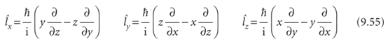
Throughout the preceding discussion, we have referred to the z-component of angular momentum (the component about an arbitrary axis, which is conventionally denotedz), and have made no reference to the x- and y-components (the components about the two axes perpendicular to z). The reason for this omission is found by examining the operators for the three components, each one being given by a term like that in eqn 9.45:
As you are invited to show in Problem 9.27, these three operators do not commute with one another:
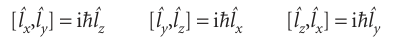
Therefore, we cannot specify more than one component (unless l = 0). In other words, lx, ly, and lz are complementary observables. On the other hand, the operator for the square of the magnitude of the angular momentum is
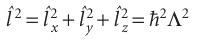
where Λ2 is the legendrian in eqn 9.51b. This operator does commute with all three components:
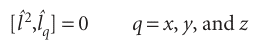
(See Problem 9.29.) Therefore, although we may specify the magnitude of the angular momentum and any of its components, if lz is known, then it is impossible to ascribe values to the other two components. It follows that the illustration in Fig. 9.38, which is summarized in Fig. 9.40a, gives a false impression of the state of the system, because it suggests definite values for the x- and y-components. A better picture must reflect the impossibility of specifying lx and ly if lz is known. The vector model of angular momentum uses pictures like that in Fig. 9.40b. The cones are drawn with side {l(l + 1)}1/2 units, and represent the magnitude of the angular momentum. Each cone has a definite projection (of ml units) on the z-axis, representing the system’s precise value of lz. The lx and ly projections, however, are indefinite. The vector representing the state of angular momentum can be thought of as lying with its tip on any point on the mouth of the cone. At this stage it should not be thought of as sweeping round the cone; that aspect of the model will be added later when we allow the picture to convey more information.
In Impact I9.1 we outlined some advantages of working in the nanometre regime. Another is the possibility of using quantum mechanical effects that render the prop erties of an assembly dependent on its size. Here we focus on the origins and con sequences of these quantum mechanical effects. Consider a sample of a metal, such as copper or gold. It carries an electrical current because the electrons are delocalized over all the atomic nuclei. That is, we may treat the movement of electrons in metals with a particle in a box model, though it is necessary to imagine that the electrons move independently of each other. Immediately, we predict from eqn 9.6 that the energy levels of the electrons in a large box, such as a copper wire commonly used to make electrical connections, form a continuum so we are justified in neglecting quantum mechanical effects on the properties of the material. However, consider a nanocrystal, a small cluster of atoms with dimensions in the nanometre scale. Again using eqn 9.6, we predict that the electronic energies are quantized and that the separation between energy levels decreases with increasing size of the cluster. This quantum mechanical effect can be observed in ‘boxes’ of any shape. For example, you are invited to show in Problem 9.39 that the energy levels of an electron in a sphere of radius R are given by
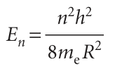
The quantization of energy in nanocrystals has important technological implications when the material is a semiconductor, in which the electrical conductivity increases with increasing temperature or upon excitation by light (see Chapter 20 for a more detailed discussion). Transfer of energy to a semiconductor increases the mobility of electrons in the material. However, for every electron that moves to a different site in the sample, a unit of positive charge, called a hole, is left behind. The holes are also mobile, so to describe electrical conductivity in semiconductors we need to consider the movement of electron–hole pairs, also called excitons, in the material. The electrons and holes may be regarded as particles trapped in a box, so eqn 9.6 can give us qualitative insight into the origins of conductivity in semiconductors. We conclude as before that only in nanocrystals are the energies of the charge carriers quantized. Now we explore the impact of energy quantization on the optical and electronic properties of semiconducting nanocrystals. Three-dimensional nanocrystals of semiconducting materials containing 103 to 105 atoms are called quantum dots. They can be made in solution or by depositing atoms on a surface, with the size of the nanocrystal being determined by the details of the synthesis (see, for example, Impact I20.2). A quantitative but approximate treatment that leads to the energy of the exciton begins with the following hamiltonian for a spherical quantum dot of radius R:
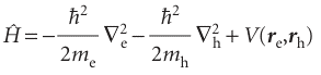
where the first two terms are the kinetic energy operators for the electron and hole (with masses me and mh, respectively), and the third term is the potential energy of interaction between electron and hole, which are located at positions re and rh from the centre of the sphere. Taking into account only the Coulomb attraction between the hole, with charge +e, and the electron, with charge −e, we write (see Chapter 9 and Appendix 3 for details):
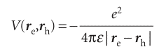
where |re − rh| is the distance between the electron and hole and ε is the permittivity of the medium (we are ignoring the effect of polarization of the medium due to the presence of charges). Solving the Schrödinger equation in this case is not a trivial task, but the final expression for the energy of the exciton, Eex, is relatively simple (see Further reading for details):
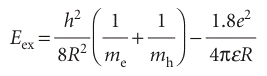
As expected, we see that the energy of the exciton decreases with increasing radius of the quantum dot. Moreover, for small R, the second term on the right of the pre ceding equation is smaller than the first term and the energy of the exciton is largely kinetic, with the resulting expression resembling the case for a particle in a sphere. The expression for Eex has important consequences for the optical properties of quantum dots. First, we see that the energy required to create mobile charge carriers and to induce electrical conductivity depends on the size of the quantum dot. The electrical properties of large, macroscopic samples of semiconductors cannot be tuned in this way. Second, in many quantum dots, such as the nearly spherical nanocrystals of cadmium selenide (CdSe), the exciton can be generated by absorption of visible light. Therefore, we predict that, as the radius of the quantum dot decreases, the excita tion wavelength increases. That is, as the size of the quantum dot varies, so does the colour of the material. This phenomenon is indeed observed in suspensions of CdSe quantum dots of different sizes. Because quantum dots are semiconductors with tunable electrical properties, it is easy to imagine uses for these materials in the manufacture of transistors. But the special optical properties of quantum dots can also be exploited. Just as the generation of an electron–hole pair requires absorption of light of a specific wavelength, so does recombination of the pair result in the emission of light of a specific wavelength. This property forms the basis for the use of quantum dots in the visualization of biological cells at work. For example, a CdSe quantum dot can be modified by covalent attach ment of an organic spacer to its surface. When the other end of the spacer reacts specifically with a cellular component, such as a protein, nucleic acid, or membrane, the cell becomes labelled with a light-emitting quantum dot. The spatial distribution of emission intensity and, consequently, of the labelled molecule can then be measured with a microscope. Though this technique has been used extensively with organic molecules as labels, quantum dots are more stable and are stronger light emitters.
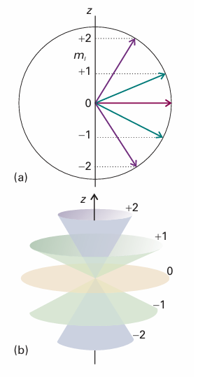
Fig. 9.40 (a) A summary of Fig. 9.38. However, because the azimuthal angle of the vector around the z-axis is indeterminate, a better representation is as in (b), where each vector lies at an unspecified azimuthal angle on its cone.
 الاكثر قراءة في مواضيع عامة في الكيمياء الفيزيائية
 اخر الاخبار
اخبار العتبة العباسية المقدسة


