Most of the functions we study in elementary calculus are described by formulas. These functions almost always possess derivatives. In fact, a portion of any first course in calculus is devoted to the development of routine methods for computing derivatives. However, not all functions possess derivatives everywhere. For example, the functions (1 + x²)/x, cot x, and sin(1/x) do not possess derivatives at x =0 no matter how they are defined at x =0.

As we progress in the study of analysis, it is important to enlarge substantially the class of functions we examine. Functions that possess derivatives everywhere form a rather restricted class; extending this class to functions that are differentiable except at a few isolated points does not enlarge it greatly. We wish to investigate significantly larger classes of functions, and to do so we introduce the notion of a continuous function.

Definitions

Suppose that f is a function from a domain D in R¹ to R¹. The function f is continuous at a if (i) the point a is in an open interval I contained in D, and (ii) for each positive number ε there is a positive number δ such that

|f(x) − f(a)| <ε whenever |x − a| <δ.

If f is continuous at each point of a set S, we say that f is continuous on S. A function f is called continuous if it is continuous at every point of its domain. The geometric significance of continuity at a point a is indicated in Figure 1.1. We recall that the inequality |f(x) − f(a)| <ε is equivalent to the double inequality

−ε<f(x) − f(a) < ε,

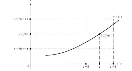
Figure 1.1 The graph of f is in the rectangle for a − δ<x<a + δ.

Or

f(a) − ε<f(x)<f(a) + ε.

Similarly, the inequality |x − a| <δ is equivalent to the two inequalities

a − δ<x<a + δ.

We construct the four lines x  a − δ, x  a + δ, y f(a) − ε, and y =f(a) + ε, as shown in Figure 1.1. The rectangle determined by these four lineshasitscenter at the point with coordinates (a, f(a)). The geometric interpretation of continuity at a point may be given in terms of this rectangle. A function f is continuous at a if for each ε> 0 there is a number δ> 0 such that the graph of  f remains within the rectangle for all x in the interval (a − δ, a + δ).

It is usually very difficult to verify continuity directly from the definition. Such verification requires that for every positive number ε we exhibit a number δ and show that the graph of f lies in the appropriate rectangle.

However, if the function f is given by a sufficiently simple expression, it is sometimes possible to obtain an explicit value for the quantity δ corresponding to a given number ε. We describe the method by means of two examples.

Example 1

Given the function

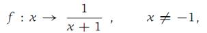
and a = 1, ε = 0.1, find a number δ such that |f(x) − f(1)| < 0.1 for |x − 1| <δ.

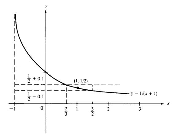
Figure 1.2

Solution. We sketch the graph of f and observe that f is decreasing for x> −1 (see Figure 1.2). The equations f(x)−f(1) = 0.1, f(x)−f(1) =−0.1 can be solved for x. We find

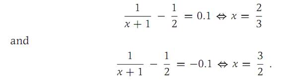
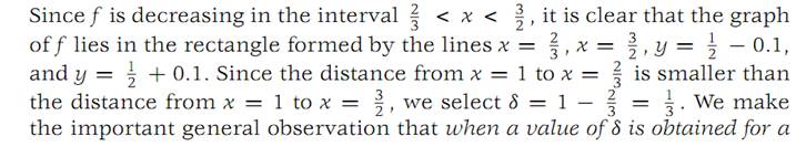
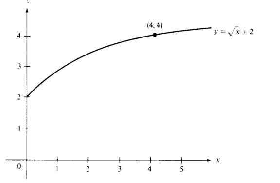
                                                  Figure 1.3

Example 2

Consider the function

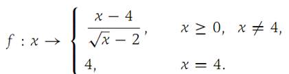
If ε = 0.01, find a δ such that |f(x) − f(4)| < 0.01 for all x such that |x − 4| <δ.

Solution.

If x ≠ 4, then factoring x − 4, we get

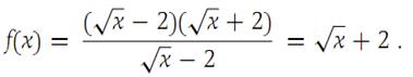
The graph of f is shown in Figure 1.3, and we observe that f is an increasing function. We solve the equations f(x) − f(4) =0.01 and f(x) − f(4) =−0.01 and obtain

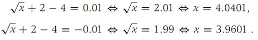
Since f  is increasing, it follows that |f(x) − f(4)| < 0.01 for 3.9601 <x< 4.0401. Selecting δ = 0.0399,

we find that |f(x) − f(4)| <ε for |x − 4| <δ.

Definition

Suppose that a and L are real numbers and f is a function from a domain D in R¹ to R¹. The number a may or may not be in the domain of f . The function f tends to L as a limit as x tends to a if (i) there is an open interval I containing a that, except possibly for the point a, is contained in D, and (ii) for each positive number ε there is a positive number δ such that

|f(x) − L| <ε whenever 0 < |x − a| <δ.

If f tends to L as x tends to a, we write

f(x) → L as x → a

and denote the number L by

(i) We see that a function f is continuous at a if and only if a is in the domain of f and f(x) → f(a) as x → a.

(ii) The condition 0 < |x − a| <δ (excluding the possibility x= a)is used rather than the condition |x−a| <δ as in the definition of continuity, since f may not be defined at a itself.

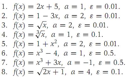
Problems

In Problems1 through 8 the functions are continuous at the value a given. In each case find a value δ corresponding to the given value of ε such that the definition of continuity is satisfied. Draw a graph.

Basic Elements of Real Analysis, Murray H. Protter, Springer, 1998 Page(21-27)

اخر الاخبار

اخبار العتبة العباسية المقدسة

معهد القرآن الكريم النسوي ينظّم سفرة دينية إلى كربلاء المقدسة لطالبات الدورات القرآنية الصيفية

العتبة العباسية المقدسة تناقش مع هيأة الإعلام والاتصالات تسهيل عمل المؤسّسات الصحفية لتغطية زيارة عاشوراء

لليوم الخامس.. العتبة العباسية المقدسة تواصل إقامة مجلس عزائها المركزي في الصحن الشريف

قسم الشؤون الدينية يفتتح موكبًا لخدمة زائري مدينة كربلاء في شهر المحرم

المزيد

الآخبار الصحية

لمن تجاوز الستين.. عليك بشرب 4 أكواب من القهوة يوميا ؟

الحليب مع العسل.. مزيج يمنحك 7 فوائد صحية

لا تبالغ في التنظيف.. قليل من "الاتساخ" قد يحمي عائلتك

دراسة تكشف علاقة خطيرة بين عمر الأم وصحة مولودها

المزيد

الآخبار التكنلوجية

هل هاتفك مراقب؟.. 5 علامات خطيرة تكشف التجسس عليك

دبي تطلق أول رحلة تجريبية للتاكسي الجوي

كيف تساعد الصيانة الوقائية في الحفاظ على كفاءة التكييف في سيارتك ؟

في ظاهرة غريبة حيرت العلماء.. كوكبنا قد يسجل أقصر يوم في التاريخ هذا الصيف!

المزيد

مواضيع ذات صلة

Elementary Theory of Metric Spaces-The Schwarz and Triangle Inequalities; Metric Spaces

Elementary Theory of Metric Spaces-Functions on Compact Sets

Elementary Theory of integration -The Darboux Integral for Functions on RN

Elementary Theory of integration -The Logarithm and Exponential Functions

Elementary Theory of integration -The Riemann Integral

Differentiation and Integration in RN-The Riemann Integral in RN

Differentiation and Integration in RN-The Darboux Integral in RN

Differentiation and Integration in RN-The Derivative in RN

Differentiation and Integration in RN-Taylor,s Theorem; Maxima and Minima

Differentiation and Integration in RN-Partial Derivatives and the Chain Rule

Basic Properties of Functions on R1 -The Heine–Borel Theorem

Basic Properties of Functions on R1 -The Cauchy Criterion