
The radial solutions
 المؤلف:
Peter Atkins، Julio de Paula
المؤلف:
Peter Atkins، Julio de Paula
 المصدر:
ATKINS PHYSICAL CHEMISTRY
المصدر:
ATKINS PHYSICAL CHEMISTRY
 الجزء والصفحة:
ص322-325
الجزء والصفحة:
ص322-325
 2025-11-24
 64
64
The radial solutions
We can anticipate some features of the shapes of the radial wavefunctions by analysing the form of Veff. The first term in eqn 10.10 is the Coulomb potential energy of the electron in the field of the nucleus. The second term stems from what in classical physics would be called the centrifugal force that arises from the angular momentum of the electron around the nucleus. When l = 0, the electron has no angular momentum, and the effective potential energy is purely Coulombic and attractive at all radii (Fig. 10.2). When l ≠ 0, the centrifugal term gives a positive (repulsive) contribution to the effective potential energy. When the electron is close to the nucleus (r ≈ 0), this repulsive term, which is proportional to 1/r2, dominates the attractive Coulombic component, which is proportional to 1/r, and the net effect is an effective repulsion of the electron from the nucleus. The two effective potential energies, the one for l = 0 and the one for l ≠ 0, are qualitatively very different close to the nucleus. However, they are similar at large distances because the centrifugal contribution tends to zero more rapidly (as 1/r2) than the Coulombic contribution (as 1/r). Therefore, we can expect the solutions with l = 0 and l ≠ 0 to be quite different near the nucleus but similar far away from it. We show in the Justification below that close to the nucleus the radial wavefunction is proportional to rl, and the higher the orbital angular momentum, the less likely the electron is to be found (Fig. 10.3). We also show that far from the nucleus all wavefunctions approach zero exponentially.
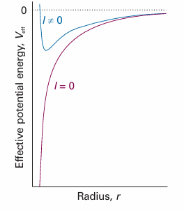
Fig. 10.2 The effective potential energy of an electron in the hydrogen atom. When the electron has zero orbital angular momentum, the effective potential energy is the Coulombic potential energy. When the electron has nonzero orbital angular momentum, the centrifugal effect gives rise to a positive contribution that is very large close to the nucleus. We can expect the l = 0 and l ≠0 wavefunctions to be very different near the nucleus.
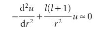
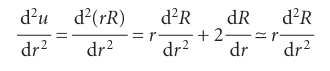
Justification 10.1 The shape of the radial wavefunction When r is very small (close to the nucleus), u ≈ 0, so the right-hand side of eqn 10.9 is zero; we can also ignore all but the largest terms (those depending on 1/r2) in eqn 10.9 and write
The solution of this equation (for r ≈ 0) is
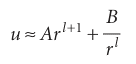
Because R = u/r, and R cannot be infinite at r = 0, we must set B = 0, and hence obtain R ≈Arl. Far from the nucleus, when r is very large, we can ignore all terms in 1/r and eqn 10.9 becomes
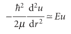
Where ≈ means ‘asymptotically equal to’. Because
this equation has the form
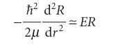
The acceptable (finite) solution of this equation (for r large) is
R ≈ e−(2µ|E|/$2)r
and the wavefunction decays exponentially towards zero as r increases.
We shall not go through the technical steps of solving the radial equation for the full range of radii, and see how the form rl close to the nucleus blends into the exponentially decaying form at great distances (see Further reading). It is sufficient to know that the two limits can be matched only for integral values of a quantum number n, and that the allowed energies corresponding to the allowed solutions are
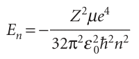
with n = 1, 2, . . . Likewise, the radial wavefunctions depend on the values of both n and l (but not on ml), and all of them have the form
R(r) = (polynomial in r) × (decaying exponential in r)
These functions are most simply written in terms of the dimensionless quantity ρ (rho), where
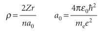
The Bohr radius, a0, has the value 52.9 pm; it is so called because the same quantity appeared in Bohr’s early model of the hydrogen atom as the radius of the electron orbit of lowest energy. Specifically, the radial wavefunctions for an electron with quantum numbers n and l are the (real) functions
Rn,l(r) = Nn,lρlL2l+1n+1(ρ)e−ρ/2
where Lis a polynomial in ρ called an associated Laguerre polynomial: it links the r ≈ 0 solutions on its left (corresponding to R ∝ ρl) to the exponentially decaying function on its right. The notation might look fearsome, but the polynomials have quite simple forms, such as 1, ρ, and 2 − ρ (they can be picked out in Table 10.1). Specifically, we can interpret the components of this expression as follows:
1 The exponential factor ensures that the wavefunction approaches zero far from the nucleus.
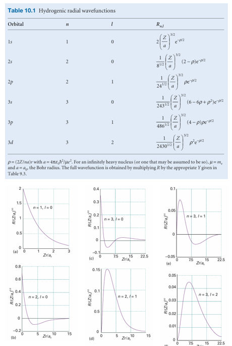
Fig. 10.4 The radial wavefunctions of the first few states of hydrogenic atoms of atomic number Z. Note that the orbitals with l = 0 have a nonzero and finite value at the nucleus. The horizontal scales are different in each case: orbitals with high principal quantum numbers are relatively distant from the nucleus.
2 The factor ρl ensures that (provided l> 0) the wavefunction vanishes at the nucleus.
3 The associated Laguerre polynomial is a function that oscillates from positive to negative values and accounts for the presence of radial nodes.
 الاكثر قراءة في مواضيع عامة في الكيمياء الفيزيائية
 اخر الاخبار
اخبار العتبة العباسية المقدسة


